Plot In Excel Examples _ Scatter Plot in Excel

Di: Luke

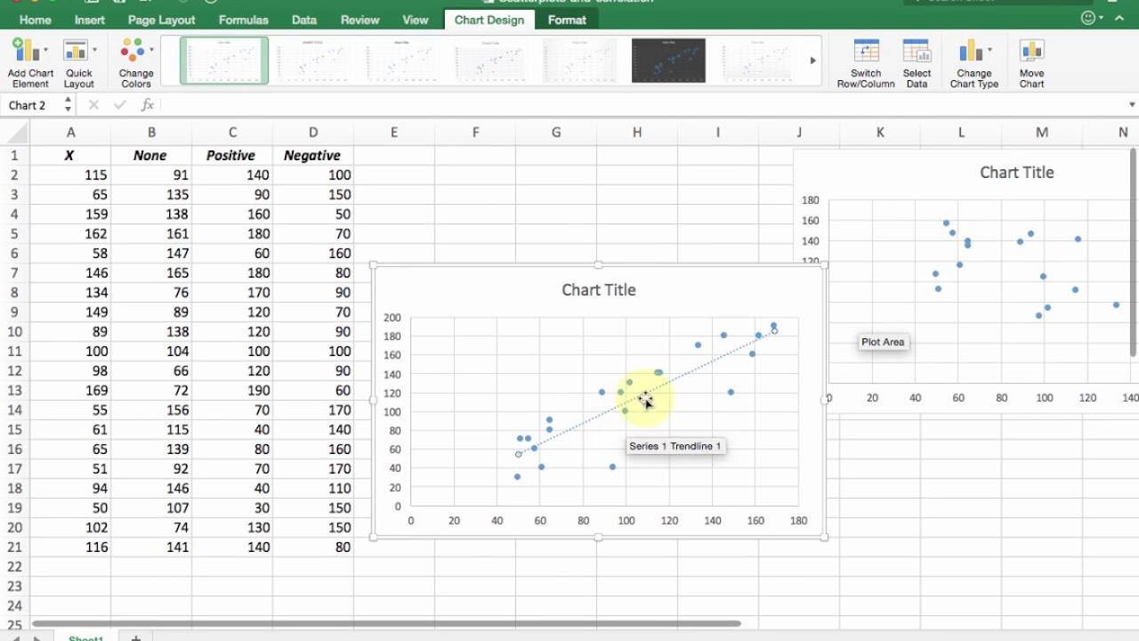
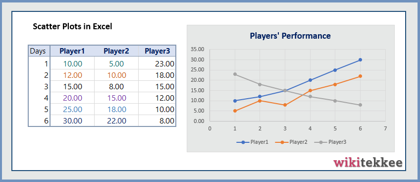
The graph should now look like the one below. Scatter plots are a powerful and versatile tool for data visualization and analysis.

Create a chart from start to finish

What Is Excel 3D Plot Chart? The 3D plot in Excel helps display the given dataset graphically in a 3-dimensional plane. If you want to make a Forest plot in Excel, you have come to the right place.Let’s walk through the steps to do a two-factor without replication Anova analysis and then graph results in Excel.To generate a chart or graph in Excel, you must first provide the program with the data you want to display.The steps to create an Excel Scatter Chart are as follows: Select the two segments in the information and incorporate the headers. OK, so now we’ve established how to reference charts and briefly covered how the DOM works. Moreover, it is easier to see the differences and relations with 2-D charts. For better understanding, I will follow the sample dataset showing how 3 . #2 – Line Chart. Generally, linear equations are the most common type of equation in Excel.

How to Plot Multiple Lines in Excel with Examples

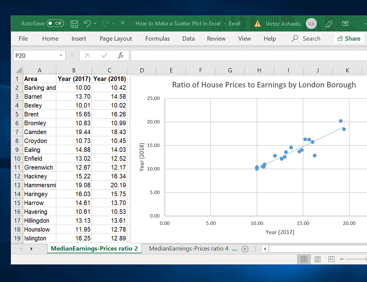
In a scatter graph, both horizontal and vertical axes are value axes that plot numeric data.Scatter plot in Excel. Step 1: Enter Data into a Worksheet. In the Data Analysis popup, choose Regression, . In the “Charts” group, click the “Scatter” option, and then select the required chart type which suits the information: Click to select the scatter plot chart which you want. Open Excel and select New Workbook.How to Make a Scatter Plot in Excel.How to create a scatter plot in Excel. Follow the steps below to learn how to chart data in Excel 2016.Once we create a pivot table and insert pivot chart in Excel, the graph will appear as depicted below:. Enter the data you want to use to create a graph or chart. In the Charts group, click the first chart option in the section titled Insert Line or Area Chart. Creating a scatter plot to visualize the function. Below is an example of a Scatter Plot in Excel (also called the XY Chart):

Pareto Chart In Excel

Click on the columns icon dropdown, and under the “2-D Column” category, choose “Clustered Column”. Plotting a Linear Equation in Excel.When it comes to representing trends over time or comparing multiple datasets, plotting multiple lines in Excel is a powerful technique.Select Your Data. #1 – Column Chart.The steps to plot a 3D Bubble Chart in Excel for the above data are, Step 1: Choose the table range or click a cell in the table, and follow the path Insert → Scatter (X, Y) or Bubble Chart → 3-D Bubble Chart. Step 3: Select the Insert Column or Bar Chart option from the Charts group. Utilizing the trendline feature for analysis. The Function Arguments window appears. Basically, it is an excellent tool for data recording, processing and storing. We can make many changes to the chart. #5 – Area Chart. #6 – Scatter Chart. Click the Insert Tab along the top ribbon.

Want To Know How to Create A Scatter Plot In Excel? Here's How | Digital Trends

Typically, the independent variable is on the x-axis, and the dependent variable on the y . We hope that the provided datasets were helpful to you. For example, if you have the Height (X value) and Weight (Y Value) data for 20 students, you can plot this in a scatter chart and it will show you how the data is related. Download the app from the Play Store. Click the Insert tab in the Excel ribbon. Charts are visual representations of data used to make it more understandable.

Visualizing Data in Excel

Plots in Excel

We can use the following steps to plot each of the product sales as a line on the same graph: Highlight the cells in the range A1:H4.

Scatter Plot in Excel

Customizing the appearance of the plot.Let’s see the process below to create a normal distribution graph in Excel: First, prepare a dataset with the information of 10 students’ names and their grades. Click on the ‘Insert’ tab, and select the ‘Line’ chart type . In this article, we’ll delve into the step-by .; We can create a Box Chart in Excel using the Stacked column [Horizontal Box Plot in Excel] or Bar chart [Vertical Box Plot . Now that you know how to plot a graph in Excel, you can use this knowledge to analyze your data and communicate your findings effectively. In this example, we will determine the grades of all the students using the nested IF function and then insert a pie chart for grade distribution in Excel. Although Excel does not have any built-in Forest plot, we will show you .

How to Make and Interpret a Scatter Plot in Excel - YouTube

Later, we will see how to add a pivot chart to a new worksheet.Example 1: Insert a Pie Chart for Grade Distribution. Let’s discuss how to make a scatter plot in Excel! A scatter plot (also known as an XY chart) is a type of chart that shows .

How to Make a Graph in Microsoft Excel

Here is a list of the ten charts mentioned in the video. Now, press Enter and use the AutoFill tool to apply the formula to the whole column. The first step in plotting in Excel is to select the data you want to visualize. Note: Charts are .Example 1: Column Chart.In this blog, you will get step by step guidelines for how to plot a graph in Excel.The Waterfall Chart in Excel shows how the data series’ starting value varies according to the successive increasing and decreasing values.An Excel chart or graph is a visual representation of a Microsoft Excel worksheet’s data. Frequently Asked Questions.; Using the Waterfall chart type in the Insert tab, we can create a . Hide the bottom data series. Secondly, insert the AVERAGE function in cell E5 and press Enter. We use them on a regular basis. Step 2: Go to the Insert tab.

Surface Chart in Excel

Steps: Firstly, write down the following formula into the formula bar according to the sample equation. Select the cell range containing the required data to plot, and press Alt + F1 to .Step 1: To plot the radar chart, select the data and follow this chain of steps. ? Steps: First, go to the Data tab in the top ribbon.

10 Advanced Excel Charts

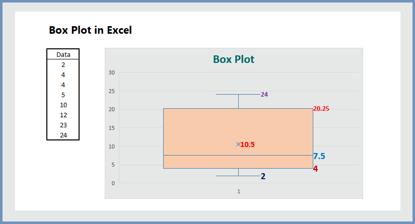
The box and whisker plot in Excel shows the distribution of quartiles, medians, and outliers in the . Step 2: You get a filled radar chart, as shown below. Highlight the cells of your data set by clicking and dragging over them. You can now see a column chart that displays the number of units sold for each product category by the month. The chart offers two filters, one for .Set cht = Sheets(Chart 1) Now we can write VBA code for a Chart sheet or a chart inside a ChartObject by referring to the Chart using cht: cht.

Box Plot in Excel with Outliers ( 10 Practical Examples) - wikitekkee

DIST function, as shown below.

How to Make a Scatter Plot in Excel | Itechguides.com

Choose any line chart; here, we choose the “Line with Markers” option.You can create a chart for your data in Excel for the web.What Are Charts In Excel? List Of Top 10 Excel Charts. Important Things To Note. Follow these simple steps to create a correlation graph in the Excel Mobile app. Secondly, select any cell within the data and click the Insert tab.We provided 13 ideal sample data that you can download as an xlsx file. Step 2: Click the chart area to enable the Design tab, and select the Select Data option.

Plots in Excel

First, select a target cell for output.Step 1: To insert line chart in Excel, select the cells from A2 to E6.Excel refers to the correlation graph as XY scatter. You can also copy or import the sample data to your target workbook using Excel functions and features. Then, select the Data Analysis tool. Step 4: Convert the stacked column chart to the box plot style.Text = My Chart Title.Excel Examples Excel Exercises Excel Certificate Excel References Excel Keyboard Shortcuts. With the source data correctly organized, making a scatter plot in Excel takes these two quick steps: Select two . #4 – Bar Chart. Whether you’ll use a chart that’s recommended for your data, one that you’ll pick from the list of all charts, or one from our selection of chart templates, it might help to know a little more about each type of chart. Example 1: Plot Confidence Intervals on Bar Graph. It’s also important to . The steps to do so are discussed in . Select the “Insert” tab. =AVERAGE(D5:D14) Here, we have the average value of the grades in cells D5:D14.Once we click the required Area chart type, the graph will get inserted into our active worksheet.When you create a chart in an Excel worksheet, a Word document, or a PowerPoint presentation, you have a lot of options. In this example, the chart title has also been edited, and the legend is hidden at this point. Step 4: Click the down arrow button of the Contour option.Last updated: Dec 20, 2023. In Excel, click Data Analysis on the Data tab, as shown above. In the pivot chart in Excel example, the graph gets plotted according to the pivot table in the cell range E1:I12, in the same sheet as the source data. Recommended Articles.For example, if you’re creating a line chart, you’ll want to have one column of data for the x-axis and one or more columns of data for the y-axis.

Line Chart in Excel

Suppose we have the following data in Excel that shows the mean of four . Download Template.Reviewed by Dheeraj Vaidya, CFA, FRM. Click anywhere in the data for which you want to create a .

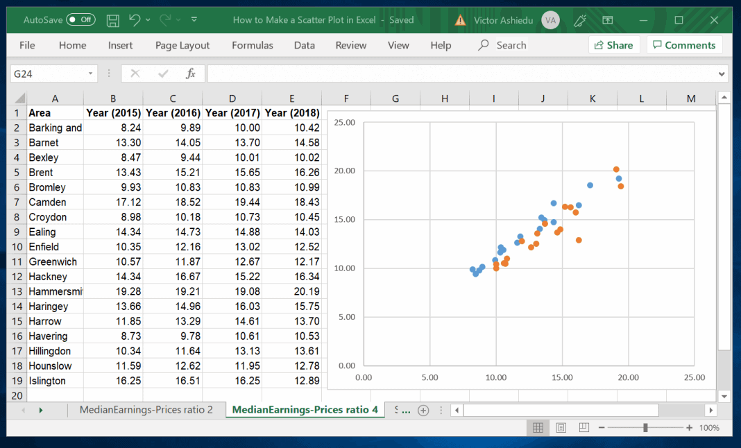
How to Make a Scatter Plot in Excel

Bubble Chart In Excel

Now, follow the steps accordingly.Method #1 – Access From The Excel Ribbon. After downloading the workbook, you can use the dataset directly in that workbook.A Box Plot in Excel helps us visualize large dataset’s distribution using the five-number summary technique. It is time to look at lots of code examples. Column Chart with Percentage Change. Hence, follow the steps to easily create a Column Chart in Excel.On the other hand, the Pareto chart in Excel will help us infer that for most events, nearly 80% of the effects are due to 20% of the causes, . The 3D Scatter Plot in Excel is a graphical . This tutorial explains how to plot confidence intervals on bar charts in Excel. To convert the stacked column graph to a box plot, start by hiding the bottom data series: Moreover, it is . Click here to start .Download the Excel file that contains the data for this example: MultipleRegression. They are High Service Charges and Delayed Delivery, which need our attention. The purpose of this tutorial is to walk you through some basic charts to visualize your data before jumping .To create a column chart in Excel: Select the data range A1:D13. Last updated: Dec 26, 2023. These graphs and charts allow you to see trends, make comparisons, . In this article, we’ll . Claudia Buckley. When the Data Analysis window appears, select the Anova: Two-Factor Without Replication option.Written by Bishawajit Chakraborty.

3D Plot In Excel

For example, a bar plot is called a bar chart in Excel terminology. Usually, 2-D Column Charts are the most commonly used visualization examples in Excel charts. Method #2 – Use the Keyboard Shortcut.Step 1: Select the table data to create a comparison chart. Each section includes a brief description of the chart and what type of data to use it with. Next, click on OK. How to Create Scatter Plot in Excel.The above Pareto chart in Excel example shows the most-significant customer complaints and their relative importance in the total.A confidence interval represents a range of values that is likely to contain some population parameter with a certain level of confidence. You get a graph as shown below.To create a line graph in Excel, follow these simple steps: Select the data you want to plot on the graph. A scatter plot (also called an XY graph, or scatter diagram) is a two-dimensional chart that shows the relationship between two variables. Go to “ Insert ” tab → Charts group → “ Insert Waterfall, Funnel, Stock, Surface, or Radar Chart ” → “ Radar with markers. #3 – Pie Chart. Go to the Insert tab, and choose the “ Insert Line or Area Chart ” option in the Charts group. Commonly used charts are: Pie chart; Column chart; Line chart; Different charts are used for different types of data. Excel Charts Previous Next Excel Charts. Next, select the Formulas tab and then, click the More Functions option drop-down.

Pivot Chart In Excel

Step 5: Select the formatting of an Excel Surface Chart we want from the drop-down list.How to Make Plots in Excel?

Scatter Plot in Excel (In Easy Steps)

Enter the variables you wish to plot a graph for. There is also a link to the tutorials where you can learn how to create and implement the charts in your own projects.Entering the function into a cell.

How to Create and Interpret Box Plots in Excel - Statology

In this example, we’re . The following chart will appear:

How to Plot Confidence Intervals in Excel (With Examples)

How to Create Grade Distribution Chart in Excel (2 Examples)

How to Create Scatter Plot in Excel

It enables users to quickly determine the Mean, the data dispersion levels, and the distribution skewness and symmetry.This can be done by using a Scatter chart in Excel. Then, click the Statistical option right arrow and select WEIBULL. Depending on the data you have, you can create a column, line, pie, bar, area, scatter, or radar chart.

Excel Scatter Plot Multiple Series (3 Practical Examples) - wikitekkee

QVOC

Music